Microsoft Excel is an essential tool for anyone who deals with data. From basic calculations to complex analysis, Excel offers a powerful arsenal of formulas and functions to help you organize, analyze, and interpret your information. But with so many options at your disposal, where do you begin?
Worry not, we’re here with the answer of this question by teaching you top 5 excel formulas you should master today!!.
This blog post will help you learn these formulas regardless of your experience level. Mastering these essentials will transform the way you interact with data in Excel, boosting your efficiency and productivity.
Are you an Excel geek?? Want to expand your learning scope?? Then there is no better place than joining the Aaru Enterprises’s Excel Using AI Workshop.
Table of Contents
Core Excel Formulas & Functions for Mastering Excel
- SUM
We start with the fundamental building block: SUM. This workhorse does exactly what its name suggests – it adds up a range of cells. Whether you’re calculating total sales figures, inventory levels, or project costs, SUM is your go-to formula.
Understanding SUM
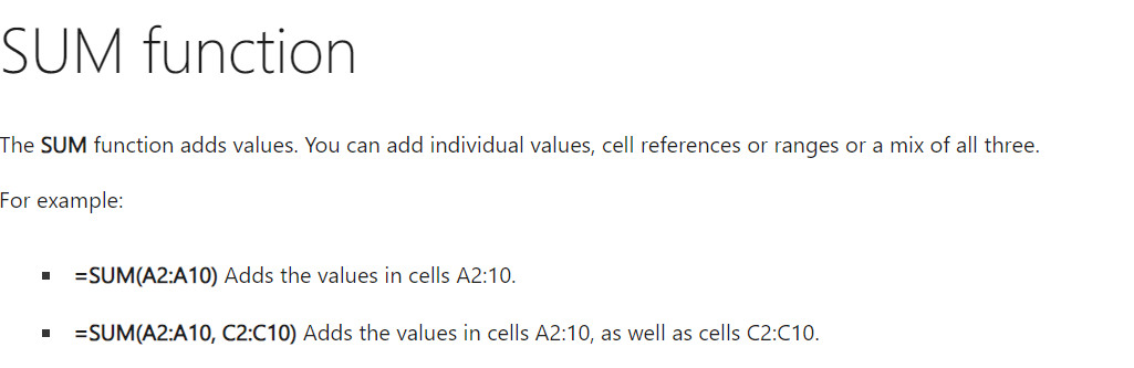
The basic syntax for the SUM function is:
Excel
=SUM(range)
Replace range with the actual cell range you want to add. For example, to add the values in cells A1 to A10, you would use:
Excel
=SUM(A1:A10)
Power Up with SUM
Handling Non-Numeric Entries: SUM ignores text entries by default. To include text values that represent numbers, you can use the VALUE function to convert them before summing. For example:
=SUM(VALUE(A1:A10))
Combining SUM with Other Formulas- SUM can be combined with other formulas for complex calculations. For instance, to calculate the total cost of items considering a discount rate, you could use
=SUM(B2:B10 * (1 – C2))
Here, B2:B10 represents the item prices, and C2 represents the discount rate (as a decimal value).
2. AVERAGE

Once you have your sum, you might want to understand what a typical value looks like. This is where AVERAGE comes in. This formula calculates the average of a set of numbers.
Calculating the Average
The AVERAGE function follows this syntax:
=AVERAGE(range)
Replace range with the cell range containing your numerical data. For example, to find the average sales figures in cells B2:B10, you would use:
=AVERAGE(B2:B10)
Beyond the Average:
Exploring Alternative Measures: While AVERAGE gives you a general idea of the “middle” value, other measures like MEDIAN can be helpful depending on your data set. MEDIAN calculates the “middle” number when your data is arranged in ascending or descending order.
Want can you get in just Rs. 99?? What if I tell you that this 99 Rs. can help you get a salary hike!! Wanna know how?? Join Aaru Enterprises’s Excel Using AI workshop.
3. COUNT & COUNTA
Need to know how many entries you have in a list? COUNT comes to the rescue! This formula simply counts the number of cells in a range that contain numbers, text, or logical values (TRUE or FALSE). But what if you only want to count cells with actual data (excluding blanks)? Enter COUNTA!
The COUNT function uses this syntax:
=COUNT(range)
Replace range with the cell range you want to analyze. For example, to count the number of entries in cells A1:A10, you would use:
=COUNT(A1:A10)
Counting with Distinction:
The COUNTA function follows a similar syntax:
=COUNTA(range)
COUNTA excludes blank cells from the count, providing a more accurate representation of data entries. For instance, to count the number of cells with data (excluding blanks) in A1:A10, you would use:
=COUNTA(A1:A10)
4. IF Statement
Excel isn’t just about number crunching; it can also perform logical evaluations. The IF function allows you to create conditional statements, enabling you to make decisions based on your data.
Conditional Logic with IF:
The basic structure of the IF statement is:
Excel
=IF(logical_test, value_if_true, value_if_false)
logical_test: This is a comparison (e.g., A1>10) that evaluates to TRUE or FALSE.
value_if_true: This is the value returned if the logical test is TRUE.
value_if_false: This
5. VLOOKUP (or HLOOKUP)
VLOOKUP is a cornerstone formula for searching and retrieving data from a table based on a specific value you provide. Imagine having a customer list with names and corresponding product codes. VLOOKUP allows you to find a specific customer’s name and return their product code from the table. HLOOKUP works similarly, but for searching data in rows instead of columns.
Alternative lookup functions like INDEX MATCH, a powerful combination for more flexible data retrieval scenarios.
Bonus Tip: Embrace Keyboard Shortcuts!
Using keyboard shortcuts can significantly speed up your Excel workflow. For example, pressing Ctrl+Shift+Enter after entering a formula in multiple cells will automatically fill the formula down the entire range, saving you time and clicks.
Conclusion
In this blog we have learned about top 5 Excel Formulas that everyone should know about. We have also seen their syntax with the help of examples.
Want more? Master Excel- the most important office tool with Aaru Enterprises’s Excel Using AI workshop in just 3 hours!!